5  Aligning and pairing the two products

To learn how the coarse product relates to the fine one, we need to compare them cell for cell on the same days. That requires three things: the two stacks on one grid, restricted to the dates they share, and then flattened into a table with one row per pixel per day. This chapter does all three and ends with a picture of the relationship the model will learn.

source(here::here("R", "setup.R"))
paths <- sih_paths()
amsr  <- load_sic_stack(paths$amsr_dir)
nsidc <- load_sic_stack(paths$nsidc_dir)

5.1 Putting both products on one grid

Both products already share a projection (EPSG:3976), so there is no reprojection to do. What differs is the grid: AMSR is 12.5 km and the Sea Ice Index is 25 km, and their extents differ slightly. We resample the coarse product onto the fine grid with bilinear interpolation, which is appropriate for a smoothly varying field like concentration. The fine AMSR grid is the target, so AMSR itself is never altered.

nsidc_aligned <- align_products(fine = amsr, coarse = nsidc)

rbind(
  amsr          = dim(amsr),
  nsidc_raw     = dim(nsidc),
  nsidc_aligned = dim(nsidc_aligned)
)

              [,1] [,2] [,3]
amsr           175  128   91
nsidc_raw       91   68   91
nsidc_aligned  175  128   91

The aligned coarse stack now has the same number of rows, columns, and layers as AMSR, so the two line up cell for cell.

This step is worth a comment, because it is the one place where this tutorial departs from the published research notebook. In that notebook the line that resamples the coarse product to 12.5 km was commented out, so the network was trained and applied on the native 25 km grid and the “12.5 km” in the output name described alignment with the AMSR extent rather than the actual cell size. We make the resample explicit, so the harmonized product genuinely sits on the 12.5 km grid and the label is accurate. The transfer function the network learns is a per-pixel value mapping either way; resampling first simply means the output grid is the fine one.

5.2 Restricting to shared dates

In general the two records only overlap for part of their span, so we pair on the dates they share. The helper stack_dates() returns each stack’s layer dates, and we keep the intersection. In the bundled sample the two products were built on the same 91 days, so all of them match, but the pattern is the one you would use on the full records where the overlap is a subset.

ad <- stack_dates(amsr)
nd <- stack_dates(nsidc_aligned)
common <- as.Date(intersect(ad, nd), origin = "1970-01-01")

amsr_ov  <- amsr[[which(ad %in% common)]]
nsidc_ov <- nsidc_aligned[[which(nd %in% common)]]
length(common)

[1] 91

5.3 Pairing pixel by pixel

Now flatten both stacks into a single table. build_pairs() reads the two stacks in the same cell-and-layer order, drops any pixel that is NA in either (land and missing data), and returns a data frame with one row per ocean pixel per shared day.

pairs <- build_pairs(fine = amsr_ov, coarse_aligned = nsidc_ov)
nrow(pairs)

[1] 1790771

head(pairs)

  nsidc amsr
1     0    0
2     0    0
3     0    0
4     0    0
5     0    0
6     0    0

That is a large training table from a modest amount of data: even this single year of every-fourth-day sampling yields well over a million paired observations, because each day contributes thousands of ocean pixels.

5.4 The relationship to be learned

Plotting the paired values against each other shows why harmonization is needed and what the model has to do. If the two products agreed perfectly, every point would fall on the dashed one-to-one line. They do not: the coarse Sea Ice Index and the fine AMSR systematically disagree, especially at intermediate concentrations near the ice edge, where the coarser footprint mixes ice and open water differently.

ggplot(pairs, aes(nsidc, amsr)) +
  geom_bin2d(bins = 80) +
  scale_fill_gradientn(colours = c("#deebf7", "#6baed6", "#2171b5", "#08306b"),
                       trans = "log10", name = "pixels") +
  geom_abline(slope = 1, intercept = 0, linetype = "dashed", color = COLORS$accent_red) +
  coord_equal(xlim = c(0, 1), ylim = c(0, 1)) +
  labs(title = "Sea Ice Index vs AMSR, paired pixels",
       x = "Sea Ice Index (25 km), SIC", y = "AMSR (12.5 km), SIC") +
  theme_bri()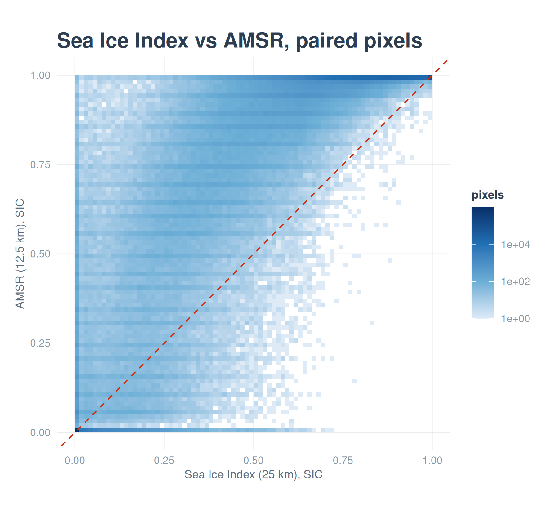

Figure 5.1: The paired relationship the model will learn, as a 2D density of the roughly 1.8 million paired pixels. The dashed line is one-to-one (perfect agreement). The cloud’s departure from it, strongest at mid-range concentrations, is the cross-sensor bias the transfer function corrects.

A quick numerical summary confirms the eye: the two products are strongly correlated but not identical, and the coarse product carries a small mean offset relative to the fine one.

c(correlation   = cor(pairs$nsidc, pairs$amsr),
  mean_bias     = mean(pairs$nsidc - pairs$amsr),
  rmse_raw      = sqrt(mean((pairs$nsidc - pairs$amsr)^2)))

correlation   mean_bias    rmse_raw 
 0.96820496 -0.06927442  0.14655607 

The next chapter fits a model to this relationship and asks whether a neural network does better than a straight line.