source(here::here("R", "setup.R"))
suppressMessages(library(nnet))  # predict.nnet must be attached for deploy_model()
paths <- sih_paths()
amsr  <- load_sic_stack(paths$amsr_dir)
nsidc <- align_products(amsr, load_sic_stack(paths$nsidc_dir))

# Use the model trained in the previous chapter; refit it here if that chapter
# has not been run, so this one stands on its own.
model_path <- file.path(sih_work_dir(), "ann_model.rds")
if (file.exists(model_path)) {
  ann <- readRDS(model_path)
} else {
  library(nnet)
  pr  <- build_pairs(amsr, nsidc)
  set.seed(sih_config$seed)
  sub <- if (nrow(pr) > 80000) pr[sample(nrow(pr), 80000), ] else pr
  ann <- nnet(amsr ~ nsidc, data = sub, size = sih_config$ann_size,
              decay = sih_config$ann_decay, maxit = sih_config$ann_maxit,
              linout = TRUE, trace = FALSE)
}7 Deploying and validating
With a fitted transfer function in hand, harmonizing is simple: apply the model to every cell of the coarse record. In the full workflow that record is the entire 1979 to 2023 Sea Ice Index, and the call is the same one shown here applied to a larger stack. On the sample we apply it to the overlap year, which lets us check the harmonized values against the AMSR observations they are meant to match. This chapter does the deployment and then validates it three ways: an overall error number, an extent time series, and difference maps in space.
7.1 Deploying the model
deploy_model() applies the network to every cell of the coarse stack and clamps the predictions to the valid range, returning a harmonized stack on the 12.5 km grid.
harmonized <- deploy_model(ann, nsidc)
harmonized
class : SpatRaster
size : 175, 128, 91 (nrow, ncol, nlyr)
resolution : 12500, 12500 (x, y)
extent : -3312500, -1712500, 162500, 2350000 (xmin, xmax, ymin, ymax)
coord. ref. : WGS 84 / NSIDC Sea Ice Polar Stereographic South (EPSG:3976)
source(s) : memory
names : 2013-01-01, 2013-01-05, 2013-01-09, 2013-01-13, 2013-01-17, 2013-01-21, ...
min values : 0.002991, 0.002991, 0.002991, 0.002991, 0.002991, 0.002991, ...
max values : 1, 1, 1, 1, 1, 1, ...
time (days) : 2013-01-01 to 2013-12-30 (91 steps)7.2 How much did harmonization help?
The single most useful number is the pooled root-mean-square error against AMSR, before and after. Harmonization should move the coarse product substantially closer to the fine one.
data.frame(
  comparison = c("Raw Sea Ice Index vs AMSR", "Harmonized vs AMSR"),
  rmse       = round(c(sic_rmse(nsidc, amsr), sic_rmse(harmonized, amsr)), 4)
)
comparison rmse
1 Raw Sea Ice Index vs AMSR 0.1466
2 Harmonized vs AMSR 0.07457.3 Tracking ice extent through the year
A more interpretable check is total sea-ice extent, the area of all cells at or above 15 percent concentration, computed for each day. If harmonization works, the harmonized curve should sit closer to the AMSR curve than the raw Sea Ice Index does, across the whole seasonal cycle.
dates <- stack_dates(amsr)
ext_df <- data.frame(
  date                  = dates,
  `AMSR (observed)`     = sic_extent_km2(amsr),
  `Sea Ice Index (raw)` = sic_extent_km2(nsidc),
  `Harmonized`          = sic_extent_km2(harmonized),
  check.names = FALSE
) |>
  tidyr::pivot_longer(-date, names_to = "product", values_to = "extent")

ggplot(ext_df, aes(date, extent / 1e6, color = product)) +
  geom_line(linewidth = 0.7) +
  scale_color_manual(values = dataset_colors, name = NULL) +
  labs(title = "Daily sea-ice extent, validation year",
       x = NULL, y = expression("Extent (" * 10^6 * " km"^2 * ")")) +
  theme_bri() + theme(legend.position = "top")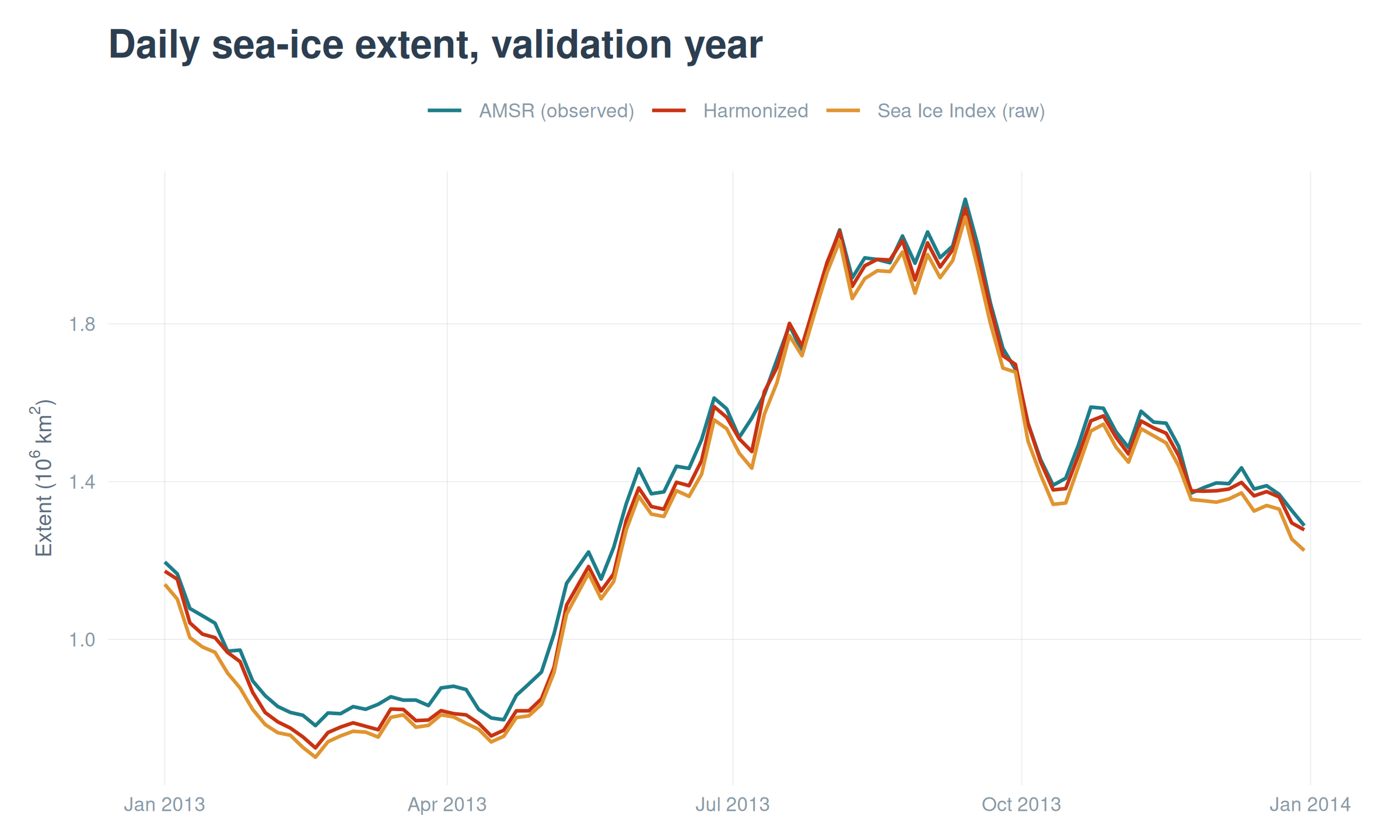
7.4 Where the products differ, in space
Extent is a single number per day, so it can hide spatial structure. Mapping the per-pixel difference between AMSR and each product on a representative day shows where the disagreement lives and whether harmonization fixes it. We draw land in black and use a diverging scale centered on zero, so blue is where AMSR reads lower than the product and orange where it reads higher.
library(patchwork)
day  <- 40
land <- terra::resample(terra::rast(paths$land_mask), amsr[[1]], method = "near")
land_df  <- subset(rast_to_df(land, "m"), !is.na(m))
land_res <- terra::res(land)

mk_diff <- function(diff_layer, title) {
  ggplot() +
    geom_tile(data = land_df, aes(x, y), fill = "black",
              width = land_res[1], height = land_res[2]) +
    geom_raster(data = rast_to_df(diff_layer, "d"), aes(x, y, fill = d)) +
    scale_fill_sic_diff() + coord_equal() +
    labs(title = title, x = NULL, y = NULL) + theme_bri_map()
}

p_raw  <- mk_diff(amsr[[day]] - nsidc[[day]],      "AMSR - raw Sea Ice Index")
p_harm <- mk_diff(amsr[[day]] - harmonized[[day]], "AMSR - harmonized")
p_raw + p_harm + plot_layout(guides = "collect")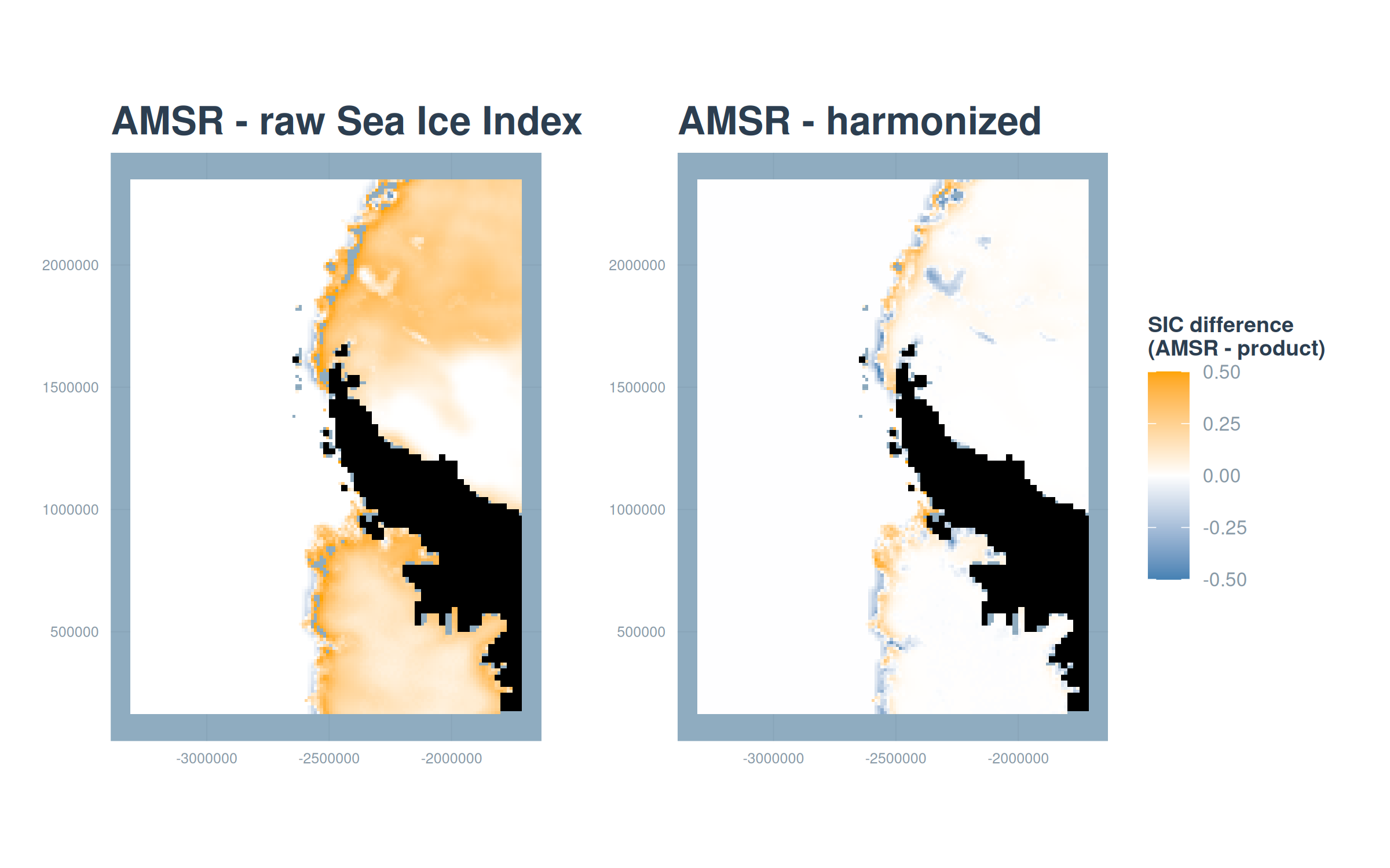
7.5 Where harmonization helps most
Finally, the per-pixel RMSE through time turns the whole validation year into one map per comparison, showing which parts of the domain harmonization improves. The reduction is largest along the marginal ice zone, the band where the coarse footprint struggles most.
rmse_raw  <- sic_rmse_pixel(amsr, nsidc)
rmse_harm <- sic_rmse_pixel(amsr, harmonized)

mk_rmse <- function(r, title) {
  ggplot() +
    geom_tile(data = land_df, aes(x, y), fill = "grey20",
              width = land_res[1], height = land_res[2]) +
    geom_raster(data = rast_to_df(r, "rmse"), aes(x, y, fill = rmse)) +
    scale_fill_viridis_c(option = "magma", direction = -1, limits = c(0, NA),
                         name = "RMSE", na.value = NA) +
    coord_equal() + labs(title = title, x = NULL, y = NULL) + theme_bri_map()
}
mk_rmse(rmse_raw, "Raw Sea Ice Index") + mk_rmse(rmse_harm, "Harmonized") +
  plot_layout(guides = "collect")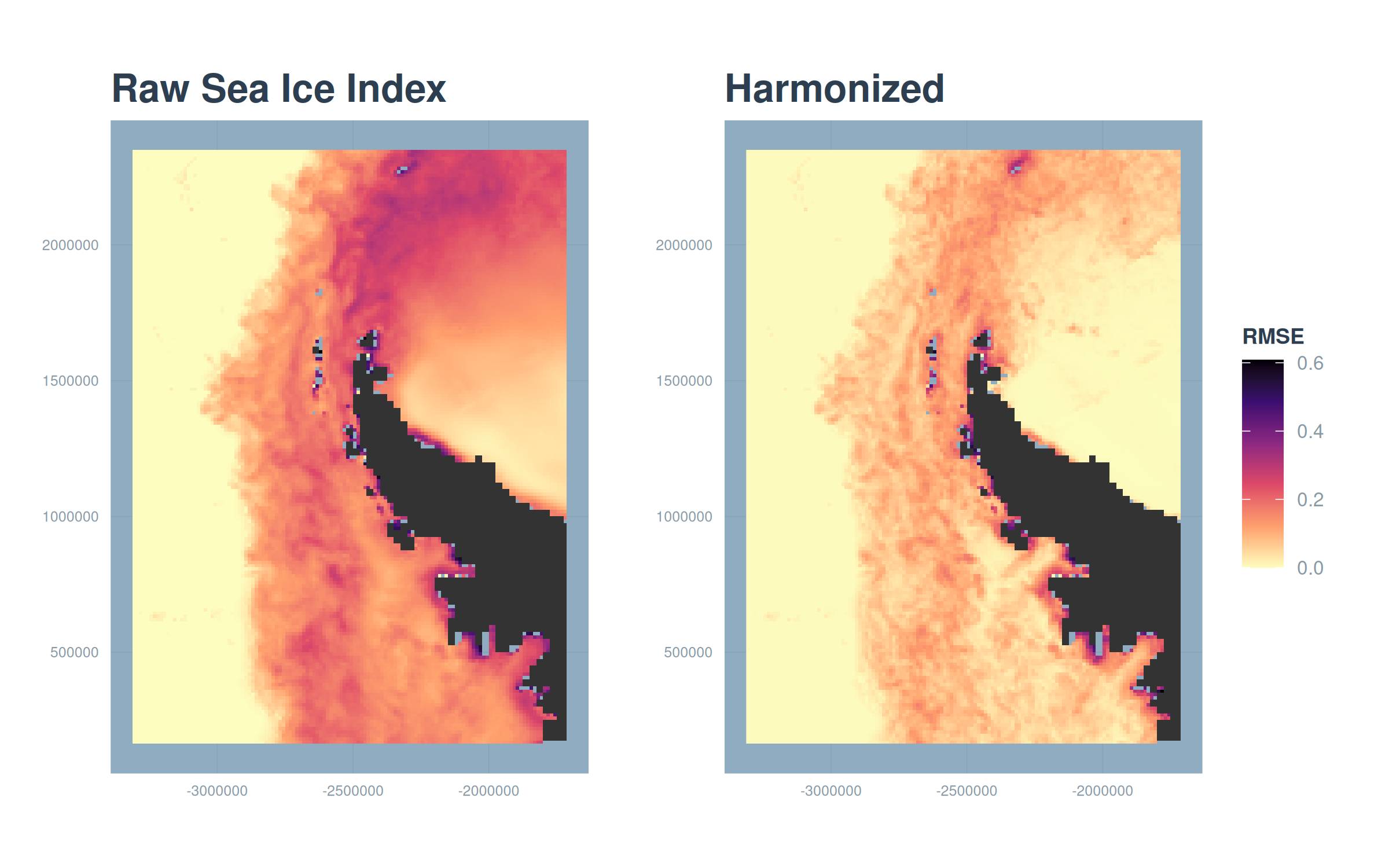
Across all three views the story is consistent. Harmonization lowers the pooled error, pulls the extent curve onto the AMSR observations, and shrinks the spatial differences most where they were largest. The harmonized product behaves like AMSR over the years we can check, which is what licenses using it to extend the fine-resolution record back to 1979. The next chapter puts that extended record to work.