8  Using the harmonized dataset

The harmonized record is now a single consistent dataset that reaches from 1979 to 2023 at 12.5 km. This chapter shows what that buys you. We compute the standard sea-ice metrics on the sample to demonstrate the code, then use the full harmonized record to estimate the long-term winter trend, which is the payoff: a fine-resolution trend across four decades that neither input product could give you alone.

source(here::here("R", "setup.R"))
suppressMessages(library(nnet))  # predict.nnet must be attached for deploy_model()
paths <- sih_paths()
amsr  <- load_sic_stack(paths$amsr_dir)
nsidc <- align_products(amsr, load_sic_stack(paths$nsidc_dir))

model_path <- file.path(sih_work_dir(), "ann_model.rds")
if (file.exists(model_path)) {
  ann <- readRDS(model_path)
} else {
  library(nnet)
  pr  <- build_pairs(amsr, nsidc); set.seed(sih_config$seed)
  sub <- if (nrow(pr) > 80000) pr[sample(nrow(pr), 80000), ] else pr
  ann <- nnet(amsr ~ nsidc, data = sub, size = sih_config$ann_size,
              decay = sih_config$ann_decay, maxit = sih_config$ann_maxit, linout = TRUE, trace = FALSE)
}
harmonized <- deploy_model(ann, nsidc)

8.1 The standard metrics

Four metrics summarize a sea-ice record. Extent is the area of cells at or above 15 percent concentration. Concentration is the mean SIC over the region. Persistence is how much of a season a given location holds ice, the proportion of days it is ice-covered. Duration is how long ice spells last, the run of consecutive ice-covered days. Extent and concentration are computed per day and summarized; persistence and duration are computed per pixel over a season.

The first two are one call each. Restricting to the austral winter (June to September) gives the season the Peninsula analysis cares about.

dates  <- stack_dates(harmonized)
winter <- which(lubridate::month(dates) %in% sih_config$winter_months)
harm_winter <- harmonized[[winter]]

c(winter_days        = length(winter),
  mean_extent_km2    = round(mean(sic_extent_km2(harm_winter))),
  mean_concentration = round(mean(sic_mean(harm_winter)), 3))

       winter_days    mean_extent_km2 mean_concentration 
            31.000        1744526.000              0.525 

Persistence is a per-pixel metric: for each cell, the fraction of winter days it is ice-covered. Mapping it shows the spatial pattern of where ice is reliable versus marginal.

persistence <- terra::app(harm_winter,
  fun = function(x) mean(x >= sih_config$ice_threshold, na.rm = TRUE))

ggplot(rast_to_df(persistence, "p"), aes(x, y, fill = p)) +
  geom_raster() +
  scale_fill_viridis_c(name = "Persistence", limits = c(0, 1), na.value = NA) +
  coord_equal() +
  labs(title = "Winter ice persistence", x = NULL, y = NULL) +
  theme_bri_map()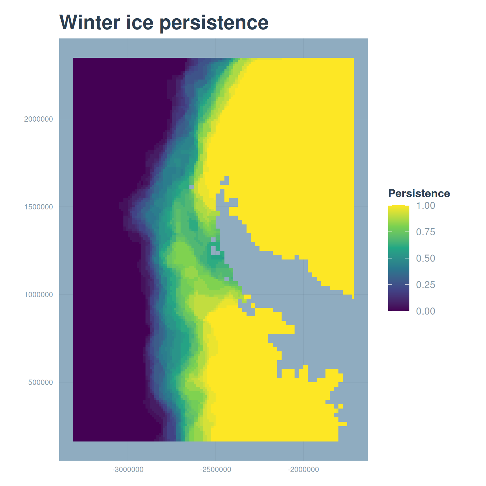

Figure 8.1: Winter ice persistence on the sample harmonized product: the fraction of winter days each cell is at or above 15 percent concentration. Values near 1 (dark) are reliably ice-covered; values near 0 are open water or the marginal ice zone.

Duration, the mean length of consecutive ice-covered spells, is defined the same way the paper computes it, with a run-length encoding of each pixel’s daily series. It needs a genuinely daily record to count consecutive days correctly, so we define it here but compute it on the full daily product rather than on the every-fourth-day sample:

mean_spell_duration <- function(x, threshold = 0.15) {
  x <- x[!is.na(x)]
  if (length(x) == 0) return(NA_real_)
  runs <- rle(x >= threshold)
  if (!any(runs$values)) return(0)
  mean(runs$lengths[runs$values])
}
duration <- terra::app(harm_winter_daily, fun = mean_spell_duration)

8.2 The long-term trend

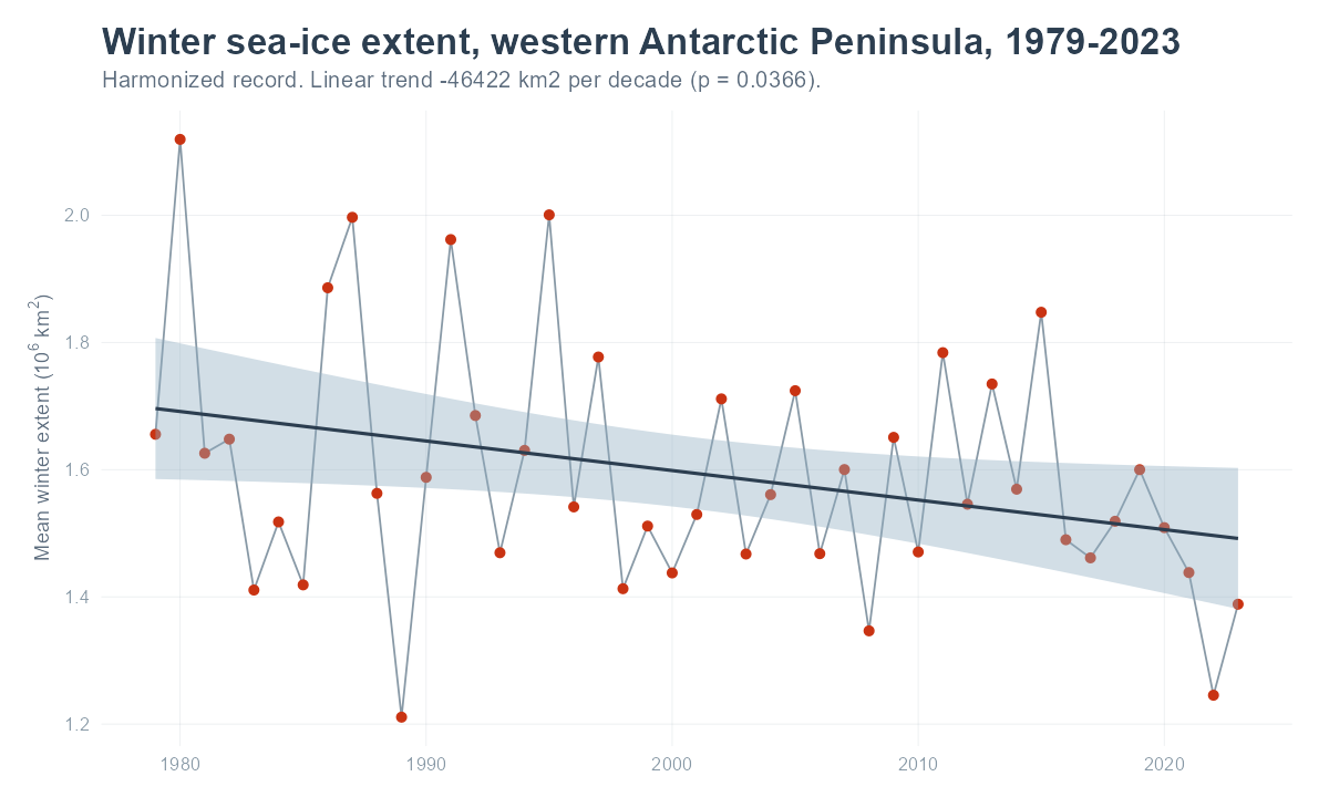
Here is the reason to harmonize. With one consistent 12.5 km record from 1979 to 2023, we can compute winter extent for every year and fit a trend. On the full record the per-year winter mean extent declines significantly over the four decades. The figure below was produced from the complete harmonized product by scripts/build_frozen.R; it does not run here, because it needs the full record rather than the sample.

Figure 8.2: Mean winter (June-September) sea-ice extent for the western Antarctic Peninsula, 1979-2023, from the harmonized product. The fitted linear trend is a decline of roughly 46,000 km2 per decade (p = 0.037). The short fine-resolution AMSR record alone could not resolve a trend this slow.

A regional average hides where the change happens. Fitting the same trend at every pixel turns the record into a map of winter concentration change, which is where the harmonized product’s spatial detail pays off.

Figure 8.3: Per-pixel trend in winter sea-ice concentration, 1979-2023, in percent per decade. Red is declining ice, blue increasing. The 12.5 km grid resolves structure along the shelf and the coast that a 25 km product would blur.

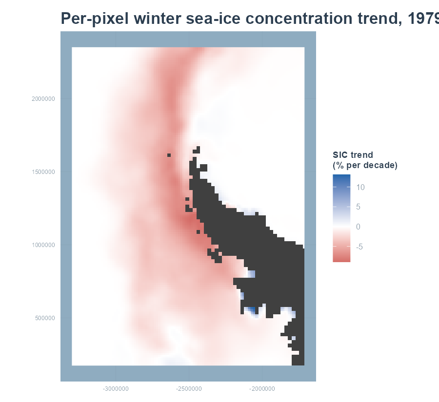
A word on the trend method. For the per-year regional series we fit an ordinary least-squares line, which is enough for a single value per year. The paper fits a generalized least-squares model with a first-order autoregressive term to the finer monthly series, because successive months are autocorrelated and ignoring that would understate the uncertainty; a Theil-Sen slope is a robust alternative when outliers are a concern. The per-pixel map uses ordinary least squares at each cell. Whichever estimator you choose, the point is the same: harmonization is what makes a 1979-2023 trend at 12.5 km possible at all, because it expresses the long coarse record in the terms of the short fine one.

The final chapter covers running this at full scale and adapting the method to other products and regions.